3. Sloppiness

The Achilles’ Heel of Research - Sloppiness

The Overarching Landscape: A Network of Traits and Challenges

Before diving deep, let’s visualize the ecosystem of clinical research. Take a look at this network graph:

Show code cell source Hide code cell source

import networkx as nx
import matplotlib.pyplot as plt

# Set seed for layout
seed = 4

# Directory structure
structure = {


    "Challenges": ["Rigor", "Sloppiness", "Error",],
    "Knowledge": ["Skills", "Challenges", "Morality", "Truth",],
    "Skills": ["Numeracy", "Literacy","Workflow",],
}

# Gentle colors for children
child_colors = ["lightgreen", "lightpink", "lightyellow",
    'lavender', 'lightcoral', 'honeydew', 'azure','lightblue', 
]

child_colors = ["lightgreen", "lightpink", "lightyellow",
    'lavender', 'lightcoral', 'honeydew', 'azure','lightblue', 
]

# 'lightsteelblue', 'lightgray', 'mintcream','mintcream', 'azure', 'linen', 'aliceblue', 'lemonchiffon', 'mistyrose'

# List of nodes to color light blue
light_blue_nodes = [ "Numeracy", "Challenges"]

G = nx.Graph()
node_colors = {}


# Function to capitalize the first letter of each word
def capitalize_name(name):
    return ' '.join(word.capitalize() for word in name.split(" "))

# Assign colors to nodes
for i, (parent, children) in enumerate(structure.items()):
    parent_name = capitalize_name(parent.replace("_", " "))
    G.add_node(parent_name)
    
    # Set the color for Skills
    if parent_name == "Knowledge":
        node_colors[parent_name] = 'lightgray'
    else:
        node_colors[parent_name] = child_colors[i % len(child_colors)]
        
    for child in children:
        child_name = capitalize_name(child.replace("_", " "))
        G.add_edge(parent_name, child_name)
        if child_name in light_blue_nodes:
            node_colors[child_name] = 'lightblue'
        else:
            node_colors[child_name] = child_colors[(i + 5) % len(child_colors)]  # You can customize the logic here to assign colors


colors = [node_colors[node] for node in G.nodes()]

# Set figure size
plt.figure(figsize=(30, 30))

# Draw the graph
pos = nx.spring_layout(G, scale=30, seed=seed)
nx.draw_networkx_nodes(G, pos, node_size=70000, node_color=colors, edgecolors='black')  # Boundary color set here
nx.draw_networkx_edges(G, pos)
nx.draw_networkx_labels(G, pos, font_size=40)
plt.show()

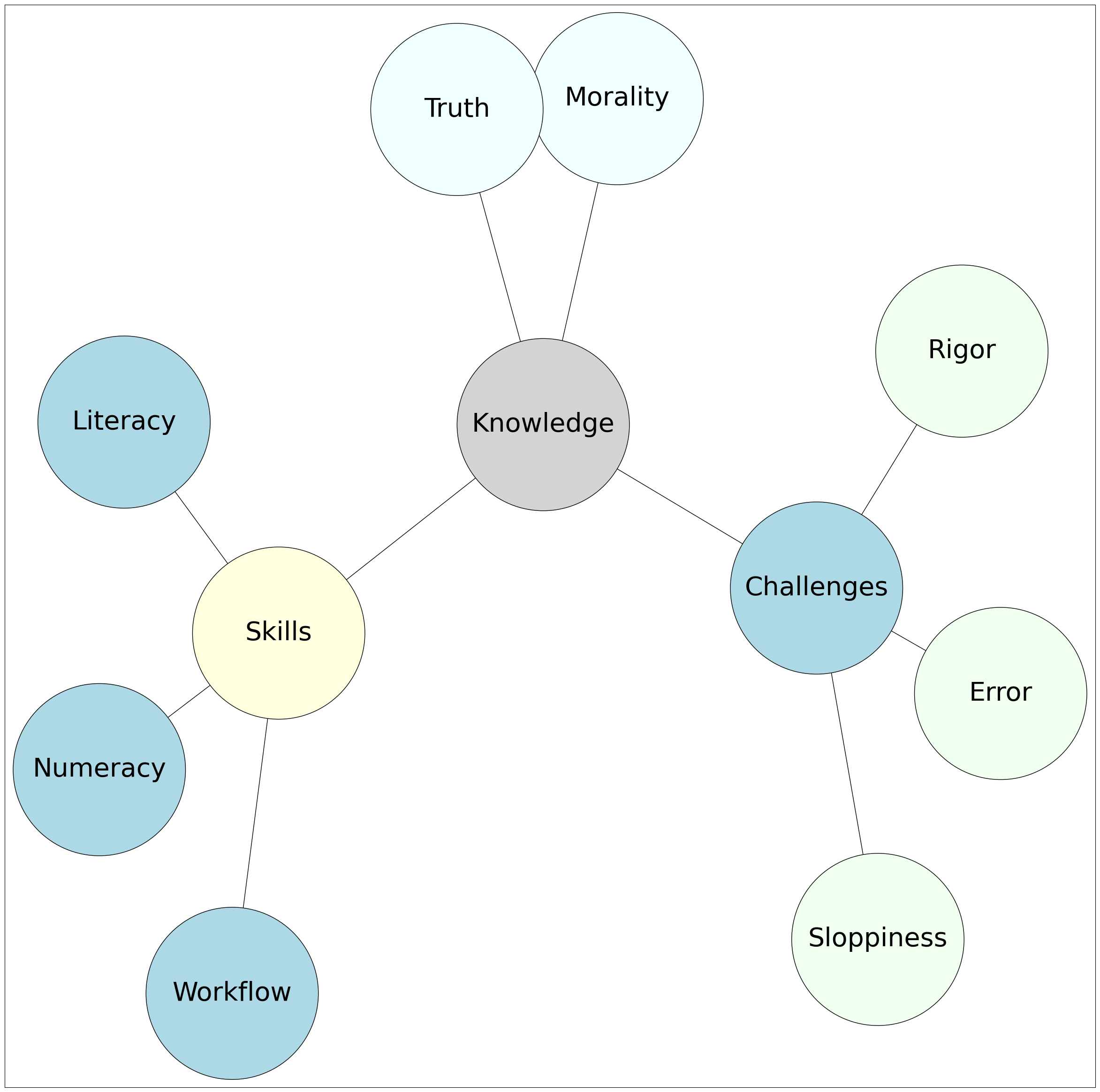
At the core, you see “Knowledge” surrounded by ‘Skills,’ ‘Challenges,’ ‘Morality,’ and ‘Truth.’ This is the universe we operate in, a multidimensional space where ‘Skills’ like literacy and numeracy combat ‘Challenges’ like rigor, sloppiness, and error. The color-coded nodes illustrate the interconnectedness and varying complexities of these components.

When Challenges Become Adversaries: The Perpetual Duel

You’re not just a researcher. You’re a warrior armed with ‘Skills,’ perpetually pitted against a formidable adversary: ‘Challenges.’ In this never-ending duel, your most sinister foe is Sloppiness. It’s the chink in your armor, the Achilles’ heel that can cause your downfall.

The Devastating Impact of Sloppiness

A single misclick, a hurried calculation, or an overlooked variable: these seemingly trivial acts of sloppiness are the landmines lurking in your research path. Consider odds ratios or 95% CIs—if contaminated by sloppiness, they don’t just mislead; they catastrophically implode the study’s integrity.

Your Weaponry Against Sloppiness: Hyper-Vigilance and Adaptability

Think of Sloppiness as a cunning rival that thrives in the murky corners of haste and neglect. To counteract it, you need a robust defense and a proactive offense.

Defense: Rigor as Your Shield

Your first line of defense is Rigor—painstaking attention to detail. With regular audits and a culture of hyper-vigilance, you build a shield that Sloppiness can’t easily penetrate.

Offense: Innovate and Adapt

On the offense, you don’t always need a high-tech arsenal. The essence is in adaptability. If advanced technology like generative adversarial networks is the special ops team in the world of data science, then in clinical research, your offense could be as straightforward yet effective as submission to the peer-review process and besting your competition (for publication and grants). It’s about leveraging the best tools and methods available to you, even if they’re metaphorical slingshots and not AI-powered machine guns.

The Eternal Recurrence: A Never-Ending Quest for Perfection

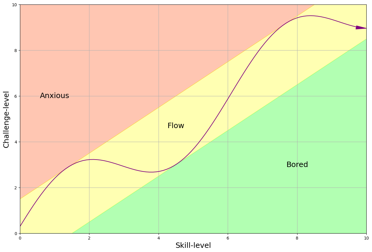
In the age-old battle between Skills and Challenges, there are no final victories. It’s a Mobius strip, an eternally recurrent challenge. Your proof of concept is not just in the outcomes but in the journey—a lifetime committed to learning, growing, innovating, and above all, overcoming sloppiness:

Show code cell source Hide code cell source

import matplotlib.pyplot as plt
import numpy as np

# Create data for the skill and challenge levels
skill_levels = np.linspace(0, 10, 100)
challenge_levels = np.linspace(0, 10, 100)

# Define the flow channel boundaries
flow_channel = skill_levels

# Adjust the phase and amplitude of the sinusoid wave
phase = np.pi / 16
amplitude = 1.5
sinusoid = flow_channel + np.sin(skill_levels + phase) * amplitude

# Define the yellow zone boundaries, making it wider
yellow_zone_low = skill_levels - 1.5  # Adjust this value to make the yellow zone wider or narrower
yellow_zone_high = skill_levels + 1.5 # Adjust this value to make the yellow zone wider or narrower

# Plotting
plt.figure(figsize=(15, 10))

# Plot the anxiety and boredom areas
plt.fill_between(skill_levels, yellow_zone_high, 10, color='orangered', alpha=0.3, label='Place/Identification', interpolate=True)
plt.fill_between(skill_levels, 0, yellow_zone_low, color='lime', alpha=0.3, label='Time/Revelation', interpolate=True)
plt.fill_between(skill_levels, yellow_zone_low, yellow_zone_high, color='yellow', alpha=0.3, label='Agent/Evolution', interpolate=True)

# Plot the sinusoid function with the diagonal as its axis
plt.plot(skill_levels, sinusoid, color='purple', linestyle='-')

# Add arrowhead to the sinusoid line
plt.arrow(skill_levels[-2], sinusoid[-2], skill_levels[-1] - skill_levels[-2], sinusoid[-1] - sinusoid[-2],
          color='purple', length_includes_head=True, head_width=0.15, head_length=0.3)

# Set plot labels and title
plt.xlabel('Skill-level', fontsize=18)
plt.ylabel('Challenge-level', rotation='vertical', fontsize=18)

# Set plot limits and grid
plt.xlim(0, 10)
plt.ylim(0, 10)
plt.grid(True)

# Set tick labels
tick_labels = ['0', '2', '4', '6', '8', '10']
plt.xticks(np.linspace(0, 10, 6), tick_labels)
plt.yticks(np.linspace(0, 10, 6), tick_labels)

# Add text annotations to label the areas without shaded background
plt.text(1, 6, 'Anxious', color='black', ha='center', va='center', fontsize=18)
plt.text(4.5, 4.7, 'Flow', color='black', ha='center', va='center', fontsize=18)
plt.text(8, 3, 'Bored', color='black', ha='center', va='center', fontsize=18)

# Display the plot
plt.show()

Takeaways: Your Battle Plan

1. Identify the Enemy: Acknowledge that Sloppiness is not just an error—it’s a volitional act with origins in boredom, relaxation, and a misguided sense of control (like the mythological Achilles), that can sabotage your work.

2. Strengthen Your Defense: Incorporate regular audits and peer reviews by submitting your work or proposaal to a friend, colleague, conference, journal, or the NIH.

3. Go on the Offense: Utilize cutting-edge tools akin to generative adversarial networks to outsmart sloppiness. Embrace this platform, Fena, and its associated resources. Step up your game and become a better researcher; get in the “flow” and enjoy the process.

By treating sloppiness as an adversary to be bested, we forge a future where every researcher becomes a stalwart guardian of integrity. With every triumph, we come one step closer to defeating our perennial foe, marching forward into a realm of more rigorous, impactful discoveries.