Show code cell source
import numpy as np
import pandas as pd
from scipy.stats import multivariate_normal, expon

def correlation_to_covariance(correlation, std_dev):
    covariance = np.outer(std_dev, std_dev) * correlation
    return covariance

def simulate_data(n=1000, study_duration=25):
    np.random.seed(42)

    # Define the correlation matrix and standard deviations
    correlation = np.array([
        [1.0, 0.5, 0.2, 0.3],
        [0.5, 1.0, 0.3, 0.4],
        [0.2, 0.3, 1.0, 0.1],
        [0.3, 0.4, 0.1, 1.0]
    ])
    std_dev = np.array([10, 15, 0.5, 5])
    cov = correlation_to_covariance(correlation, std_dev)
    mean = [60, 120, 1, 25]
    age, sbp, scr, bmi = multivariate_normal.rvs(mean=mean, cov=cov, size=n).T

    # Other variables
    hba1c = np.random.normal(5, 1, n)
    hypertension = np.random.randint(2, size=n)
    smoke = np.random.randint(2, size=n)
    racecat = np.random.choice(['Black', 'Hispanic', 'Other', 'White'], n)
    educat = np.random.choice(['High School', 'K-8', 'Some college'], n)
    male = np.random.randint(2, size=n)

    # Simulate time to kidney failure using a log-normal distribution
    median_time_to_failure = 15
    mean_time_to_failure = 19
    sigma = np.sqrt(np.log(mean_time_to_failure**2 / median_time_to_failure**2))
    mu = np.log(median_time_to_failure)
    time_to_kidney_failure = np.random.lognormal(mean=mu, sigma=sigma, size=n)
    time_to_kidney_failure = np.clip(time_to_kidney_failure, 0.1, 30)

    # Simulate censoring times using an exponential distribution
    censoring_times = expon.rvs(scale=study_duration, size=n)
    observed_times = np.minimum(time_to_kidney_failure, censoring_times)
    status = (time_to_kidney_failure <= censoring_times).astype(int)

    # Create a DataFrame
    df = pd.DataFrame({
        'age': age,
        'sbp': sbp,
        'scr': scr,
        'bmi': bmi,
        'hba1c': hba1c,
        'hypertension': hypertension,
        'smoke': smoke,
        'race': racecat,
        'education': educat,
        'male': male,
        'time_to_failure': observed_times,
        'status': status
    })

    return df

# Simulate the data
df = simulate_data()

# Save to CSV
df.to_csv("simulated_data_with_censoring.csv", index=False)

# Print summaries
print(df.describe())
               age          sbp          scr          bmi        hba1c  \
count  1000.000000  1000.000000  1000.000000  1000.000000  1000.000000
mean     59.973979   119.472001     1.009669    24.897981     4.950726
std       9.856352    14.501902     0.503815     5.057554     0.992380
min      30.326603    64.838818    -0.466847     8.899264     1.823296
25%      53.111644   109.675974     0.660291    21.504805     4.317395
50%      60.174003   119.788775     1.013048    24.949501     4.981758
75%      66.429221   128.751981     1.347884    28.092598     5.639123
max      97.106483   164.260059     2.739422    40.477585     8.112910

       hypertension        smoke        male  time_to_failure       status
count   1000.000000  1000.000000  1000.00000      1000.000000  1000.000000
mean       0.505000     0.493000     0.50000        11.227176     0.512000
std        0.500225     0.500201     0.50025         7.928697     0.500106
min        0.000000     0.000000     0.00000         0.025571     0.000000
25%        0.000000     0.000000     0.00000         5.141288     0.000000
50%        1.000000     0.000000     0.50000         9.519271     1.000000
75%        1.000000     1.000000     1.00000        15.464865     1.000000
max        1.000000     1.000000     1.00000        30.000000     1.000000
Show code cell source
# !pip install lifelines

import pandas as pd
from lifelines import CoxPHFitter

# Convert categorical variables to dummies
df_dummies = pd.get_dummies(df, columns=['race', 'education'], drop_first=True)

# Instantiate the Cox Proportional Hazards model
cph = CoxPHFitter()

# Fit the model to the data
cph.fit(df_dummies, duration_col='time_to_failure', event_col='status')

# Print the summary table, which includes HRs and 95% CIs
cph.print_summary()

# Coefficient matrix (log hazard ratios)
coefficients = cph.params_
print("Coefficient Matrix:")
print(coefficients)

# Variance-covariance matrix
variance_covariance_matrix = cph.variance_matrix_
print("Variance-Covariance Matrix:")
print(variance_covariance_matrix)
| model | lifelines.CoxPHFitter |
|---|---|
| duration col | 'time_to_failure' |
| event col | 'status' |
| baseline estimation | breslow |
| number of observations | 1000 |
| number of events observed | 512 |
| partial log-likelihood | -2866.24 |
| time fit was run | 2023-08-17 22:04:12 UTC |
| coef | exp(coef) | se(coef) | coef lower 95% | coef upper 95% | exp(coef) lower 95% | exp(coef) upper 95% | cmp to | z | p | -log2(p) | |
|---|---|---|---|---|---|---|---|---|---|---|---|
| age | -0.01 | 0.99 | 0.01 | -0.02 | -0.00 | 0.98 | 1.00 | 0.00 | -2.65 | 0.01 | 6.96 |
| sbp | -0.00 | 1.00 | 0.00 | -0.01 | 0.01 | 0.99 | 1.01 | 0.00 | -0.08 | 0.94 | 0.09 |
| scr | 0.13 | 1.14 | 0.09 | -0.06 | 0.31 | 0.94 | 1.37 | 0.00 | 1.36 | 0.18 | 2.51 |
| bmi | 0.01 | 1.01 | 0.01 | -0.01 | 0.03 | 0.99 | 1.03 | 0.00 | 0.61 | 0.54 | 0.88 |
| hba1c | -0.05 | 0.95 | 0.04 | -0.13 | 0.04 | 0.88 | 1.04 | 0.00 | -1.06 | 0.29 | 1.80 |
| hypertension | 0.10 | 1.11 | 0.09 | -0.07 | 0.28 | 0.93 | 1.32 | 0.00 | 1.12 | 0.26 | 1.94 |
| smoke | -0.03 | 0.97 | 0.09 | -0.20 | 0.15 | 0.82 | 1.16 | 0.00 | -0.30 | 0.76 | 0.39 |
| male | -0.01 | 0.99 | 0.09 | -0.19 | 0.17 | 0.83 | 1.18 | 0.00 | -0.10 | 0.92 | 0.12 |
| race_Hispanic | 0.18 | 1.20 | 0.13 | -0.06 | 0.43 | 0.94 | 1.54 | 0.00 | 1.48 | 0.14 | 2.84 |
| race_Other | 0.20 | 1.23 | 0.12 | -0.04 | 0.44 | 0.96 | 1.56 | 0.00 | 1.66 | 0.10 | 3.36 |
| race_White | 0.10 | 1.11 | 0.13 | -0.14 | 0.35 | 0.87 | 1.42 | 0.00 | 0.83 | 0.41 | 1.29 |
| education_K-8 | -0.17 | 0.85 | 0.11 | -0.38 | 0.05 | 0.68 | 1.05 | 0.00 | -1.49 | 0.14 | 2.87 |
| education_Some college | -0.13 | 0.88 | 0.11 | -0.34 | 0.08 | 0.71 | 1.08 | 0.00 | -1.23 | 0.22 | 2.18 |
| Concordance | 0.55 |
|---|---|
| Partial AIC | 5758.48 |
| log-likelihood ratio test | 17.00 on 13 df |
| -log2(p) of ll-ratio test | 2.33 |
Coefficient Matrix:
covariate
age                      -0.013337
sbp                      -0.000274
scr                       0.128553
bmi                       0.006206
hba1c                    -0.046943
hypertension              0.100960
smoke                    -0.027003
male                     -0.008717
race_Hispanic             0.184603
race_Other                0.203355
race_White                0.104264
education_K-8            -0.165335
education_Some college   -0.132012
Name: coef, dtype: float64
Variance-Covariance Matrix:
covariate                    age       sbp       scr       bmi         hba1c  \
covariate
age                     0.000025 -0.000006 -0.000075 -0.000007  8.126299e-06
sbp                    -0.000006  0.000013 -0.000071 -0.000011 -2.379526e-06
scr                    -0.000075 -0.000071  0.008991 -0.000013  6.076963e-05
bmi                    -0.000007 -0.000011 -0.000013  0.000104  1.701619e-05
hba1c                   0.000008 -0.000002  0.000061  0.000017  1.945850e-03
hypertension            0.000006  0.000003  0.000398 -0.000026 -4.582618e-05
smoke                  -0.000023 -0.000018 -0.000176 -0.000017 -5.294871e-07
male                   -0.000056  0.000019  0.000426  0.000024  1.603505e-04
race_Hispanic           0.000006  0.000003  0.000451  0.000048  4.355287e-04
race_Other             -0.000051 -0.000019  0.000118  0.000004  1.328256e-04
race_White             -0.000036  0.000021  0.000219 -0.000015  3.049609e-04
education_K-8           0.000022 -0.000043 -0.000194  0.000050 -3.356481e-05
education_Some college -0.000008 -0.000050  0.000051  0.000059 -3.188334e-04

covariate               hypertension         smoke      male  race_Hispanic  \
covariate
age                         0.000006 -2.290813e-05 -0.000056       0.000006
sbp                         0.000003 -1.776325e-05  0.000019       0.000003
scr                         0.000398 -1.757945e-04  0.000426       0.000451
bmi                        -0.000026 -1.681884e-05  0.000024       0.000048
hba1c                      -0.000046 -5.294871e-07  0.000160       0.000436
hypertension                0.008060 -7.885446e-04  0.000035      -0.000100
smoke                      -0.000789  8.103736e-03  0.000485       0.000492
male                        0.000035  4.848158e-04  0.008091      -0.000219
race_Hispanic              -0.000100  4.924759e-04 -0.000219       0.015657
race_Other                 -0.000769  3.214313e-04  0.000412       0.007145
race_White                  0.000502  6.153204e-04  0.000814       0.007237
education_K-8              -0.000009  1.486314e-04  0.000085      -0.000140
education_Some college     -0.000223  2.258767e-04 -0.000302      -0.000318

covariate               race_Other  race_White  education_K-8  \
covariate
age                      -0.000051   -0.000036       0.000022
sbp                      -0.000019    0.000021      -0.000043
scr                       0.000118    0.000219      -0.000194
bmi                       0.000004   -0.000015       0.000050
hba1c                     0.000133    0.000305      -0.000034
hypertension             -0.000769    0.000502      -0.000009
smoke                     0.000321    0.000615       0.000149
male                      0.000412    0.000814       0.000085
race_Hispanic             0.007145    0.007237      -0.000140
race_Other                0.015080    0.007204      -0.000875
race_White                0.007204    0.015962       0.000017
education_K-8            -0.000875    0.000017       0.012373
education_Some college   -0.001031   -0.000184       0.005783

covariate               education_Some college
covariate
age                                  -0.000008
sbp                                  -0.000050
scr                                   0.000051
bmi                                   0.000059
hba1c                                -0.000319
hypertension                         -0.000223
smoke                                 0.000226
male                                 -0.000302
race_Hispanic                        -0.000318
race_Other                           -0.001031
race_White                           -0.000184
education_K-8                         0.005783
education_Some college                0.011580
Show code cell source
from lifelines import KaplanMeierFitter
import matplotlib.pyplot as plt
# Instantiate the KaplanMeierFitter
kmf = KaplanMeierFitter()
# Fit the data into the model
kmf.fit(df['time_to_failure'], event_observed=df['status'])
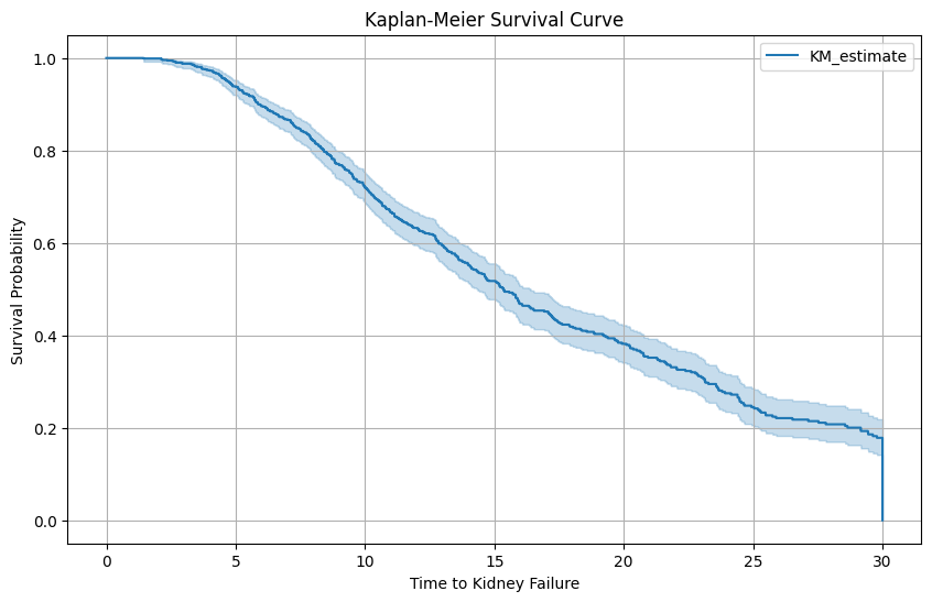
# Plot the Kaplan-Meier survival curve
plt.figure(figsize=(10, 6))
kmf.plot()
plt.title('Kaplan-Meier Survival Curve')
plt.xlabel('Time to Kidney Failure')
plt.ylabel('Survival Probability')
plt.grid(True)
plt.savefig('1_min_KM.png')
plt.show()
Show code cell source
from lifelines import KaplanMeierFitter
import matplotlib.pyplot as plt
# Instantiate the KaplanMeierFitter
kmf = KaplanMeierFitter()
# Fit the data into the model
kmf.fit(df['time_to_failure'], event_observed=df['status'])
# Get the survival function
survival_function = kmf.survival_function_
# Compute 1 minus the survival function
complement_survival_function = 1 - survival_function
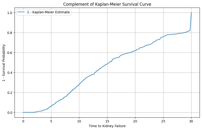
# Plot the complement of the Kaplan-Meier survival curve
plt.figure(figsize=(10, 6))
plt.plot(complement_survival_function, label='1 - Kaplan-Meier Estimate')
plt.title('Complement of Kaplan-Meier Survival Curve')
plt.xlabel('Time to Kidney Failure')
plt.ylabel('1 - Survival Probability')
plt.legend()
plt.grid(True)
plt.savefig('1_min_KM.png')
plt.show()